Cartogram Chart: Definition, Types, and Best Practices

Cartogram charts resize map regions so their area matches data values. That simple trick can change what people notice first, and what they ignore. This article explains how cartograms work, when they outperform standard maps, the data requirements for building them, and how to avoid pitfalls that can send your audience to the wrong conclusion.
What is a cartogram chart?
Picture a map of the US where Texas looks oddly small and New Jersey looks enormous. That’s a cartogram.
A cartogram chart is a map where region sizes have been distorted to represent data values instead of actual land area. The distortion is intentional. It pushes you to see which regions matter for a specific variable like population, revenue, or votes.
Standard maps can mislead you in a specific way: They make big geographic areas feel important simply because they take up visual space. A cartogram flips that around and resizes each region so area corresponds to the metric you are most interested in.
In BI, cartogram charts typically show up in dashboards as an interactive way to tell a geographic story. For a data analyst or BI specialist, they’re often the difference between “here’s a map” and “here’s where the business is actually happening.” The terms “cartogram map” and “cartogram chart” mean the same thing. You’ll see both in the wild.
When to use a cartogram chart
When discussion of the geographic size would steer the conversation in the wrong direction, a cartogram earns its spot.
Election maps are the classic example. Rural areas cover enormous expanses of land but contain relatively few voters, while dense urban states punch far above their geographic weight.
Cartograms work best when your audience already knows the base geography. A US audience will recognize a distorted map of American states. A European audience will recognize warped country boundaries. Show a cartogram of Indonesian provinces to someone unfamiliar with that geography and you’ll get confusion, not insight. And honestly, that’s the part most guides skip over. Familiarity with the base map isn’t a nice-to-have. It’s the whole thing.
If you spend a lot of time explaining maps to stakeholders, this is one of the rare visuals that can save you time. Less “why is that state so big?” and more “oh, that’s where the value is.”
Here are the situations where cartograms usually shine:
- Executive presentations: When you need stakeholders to immediately grasp which regions drive the most value (especially in board or leadership decks)
- Public policy storytelling: When you want to show that population or economic activity doesn’t match land area
- Resource allocation decisions: When you need to justify shifting investment from geographically large but low-value territories
Skip cartograms when precise location matters. If someone wants to know where to build a warehouse or how far apart two regions are, the distortion will mislead them.
Also, if your data variable already correlates with land area (like agricultural output in farming regions), the map won’t change much. That can leave people wondering why they’re looking at a cartogram in the first place.
Data requirements for cartogram charts
The chart is only as clean as the join.
At minimum, you need two things: a geographic identifier for each region and a numeric value to encode as area. And yes, “region” has to mean the same thing all the way through (state vs county vs sales territory). Mixing levels is one of the fastest ways to end up with a cartogram that looks plausible and is completely wrong.
The geographic identifier must match a boundary file or shapefile. This could be country codes, state Federal Information Processing Standards (FIPS) codes, or district IDs. The numeric value is whatever you want the area to represent, like population, revenue, votes, or inventory count.
If you’re building cartogram charts inside a governed BI environment, metric definitions matter more than most people expect. Poor-quality data can lead to a 20 percent decrease in productivity. On a cartogram, that lost time often shows up as avoidable rework, people arguing about territory totals, and teams rebuilding the same map with different numbers.
You can add a secondary variable for color encoding, which turns the cartogram into a bivariate display. Size might show population while color shows income level. Just don’t pick two variables that tell competing stories (like area for totals and color for a different total on a wildly different scale). The viewer won’t know which signal to trust, and they’ll stop trusting either.
Five regions is roughly the minimum for a cartogram to make sense. Fewer than that, and a simple bar chart communicates the ranking more clearly without the geographic overhead.
Some data conditions will break the visualization even if it technically renders. If one region dominates your data set (say, one country has 10 times the value of all others combined), that region will balloon to fill the screen while everything else collapses into unreadable slivers. Similarly, if most regions have zero or near-zero values, the map will look broken rather than informative.
Data quality issues (which Gartner estimates cost organizations $12.9 million annually) can also sneak in through the join. For cartograms, the practical impact is simple: One bad join can make a territory disappear, duplicate, or get the wrong value, and the distortion makes that error feel “true.” If your region IDs don’t match cleanly to the boundary file, you’ll get missing or duplicated regions. Data engineers tend to spot this first because they live in the land of pipeline validation and “why is this territory showing up twice?”
When your data doesn’t fit these requirements, a choropleth map works better for rate-based data, and a bubble map overlay works better for totals on accurate geography.
Why cartogram charts exist
Big shapes grab attention, even when they shouldn’t.
Geographic maps encode land area, which is often irrelevant for business and policy questions. When you display regional revenue on a standard US map, states like Texas and California dominate visually even if New Jersey and Massachusetts generate more revenue. Executives scan the largest shapes first. Geographic size hijacks attention. It’s a perceptual bug, and cartograms are the fix.
Cartograms invert this problem. Making area proportional to the variable that matters forces viewers to confront magnitude differences directly. The distortion is the message.
But there’s a cost: Cartograms sacrifice the ability to locate regions precisely. Viewers who don’t recognize the base geography will struggle to identify which blob is which. That’s acceptable when the goal is comparative magnitude (which regions matter most?) but unacceptable when the goal is spatial navigation (where should we open the next warehouse?).
How cartogram charts reframe the question
What changes isn’t the data. It’s the question the data seems to be asking.
Instead of prompting, “Where is this happening?” a cartogram reframes the question to “Who has the most of this variable?” This reframing is deliberate.
Without the chart, people default to geographic intuition. They assume large countries have large populations, large states have large economies, large districts have large voter bases. Those assumptions break all the time. A cartogram makes the break visible.
Teams can easily become overconfident with what they think is important: focusing on regions that are growing and deprioritizing regions that are shrinking. It works well for resource allocation and market sizing. But it gets risky when shrinking regions still matter for strategic reasons, like regulatory hubs or emerging markets. There’s no clean answer here. You have to know what you’re optimizing for before you let the map tell you what to care about.
A standard map treats every square mile equally. But a cartogram treats each data unit equally. That shift is the whole point.
How to read a cartogram chart
Start with what your eyes do anyway: They go to the biggest shapes.
Viewers scan for the largest regions and mentally rank them before reading labels or legends. That’s fine for ordering. It’s shaky for precise comparison.
Misinterpretation happens in predictable ways. Viewers assume adjacency relationships are preserved when they may not be (in some cartogram types, regions float freely). Viewers assume they can estimate precise values from area, but human perception of area is notoriously inaccurate. Size was identified as the most common visualization pitfall in a systematic review of scientific publications. For cartograms, that finding translates to a very real problem: People will overread small area differences and miss the safer conclusion, which is usually rank and relative magnitude.
If you’re sharing a cartogram chart in a dashboard with filters (time period, product line, territory owner), double-check what state the dashboard opens in. A cartogram that defaults to “last quarter” can tell a very different story than one set to year-to-date.
A solid reading order looks like this:
- Find a few anchor regions you recognize (largest country, your home state, a familiar landmark).
- Note which regions expanded and which shrank relative to your mental map.
- Read the legend to confirm what variable is encoded as area.
- Resist estimating precise values from shape size.
- Check whether adjacency is preserved before drawing conclusions about regional relationships.
Types of cartogram charts
Not all cartograms distort geography the same way. Choosing one comes down to recognition, adjacency, and how aggressive the distortion should be.
Contiguous cartograms
Borders stay connected, but shapes stretch and warp. Adjacency is preserved, so viewers can trace borders and recognize regional clusters. Use these when your audience knows the base geography well.
Extreme value differences can distort shapes beyond recognition. Small regions surrounded by large ones may become unreadable slivers, and if you don’t label those slivers, people will confidently guess wrong. You’ll notice this problem most in data sets where one or two regions dominate the rest by an order of magnitude.
Non-contiguous cartograms
Same shapes, different sizes, and now with gaps.
Regions retain their original shapes but resize and float independently, separated by space. Shapes stay recognizable, but adjacency is lost. Use these when shape recognition matters more than regional clustering. If someone starts reading the gaps as distance, the map is no longer doing its job, so be explicit about what the spacing does not mean.
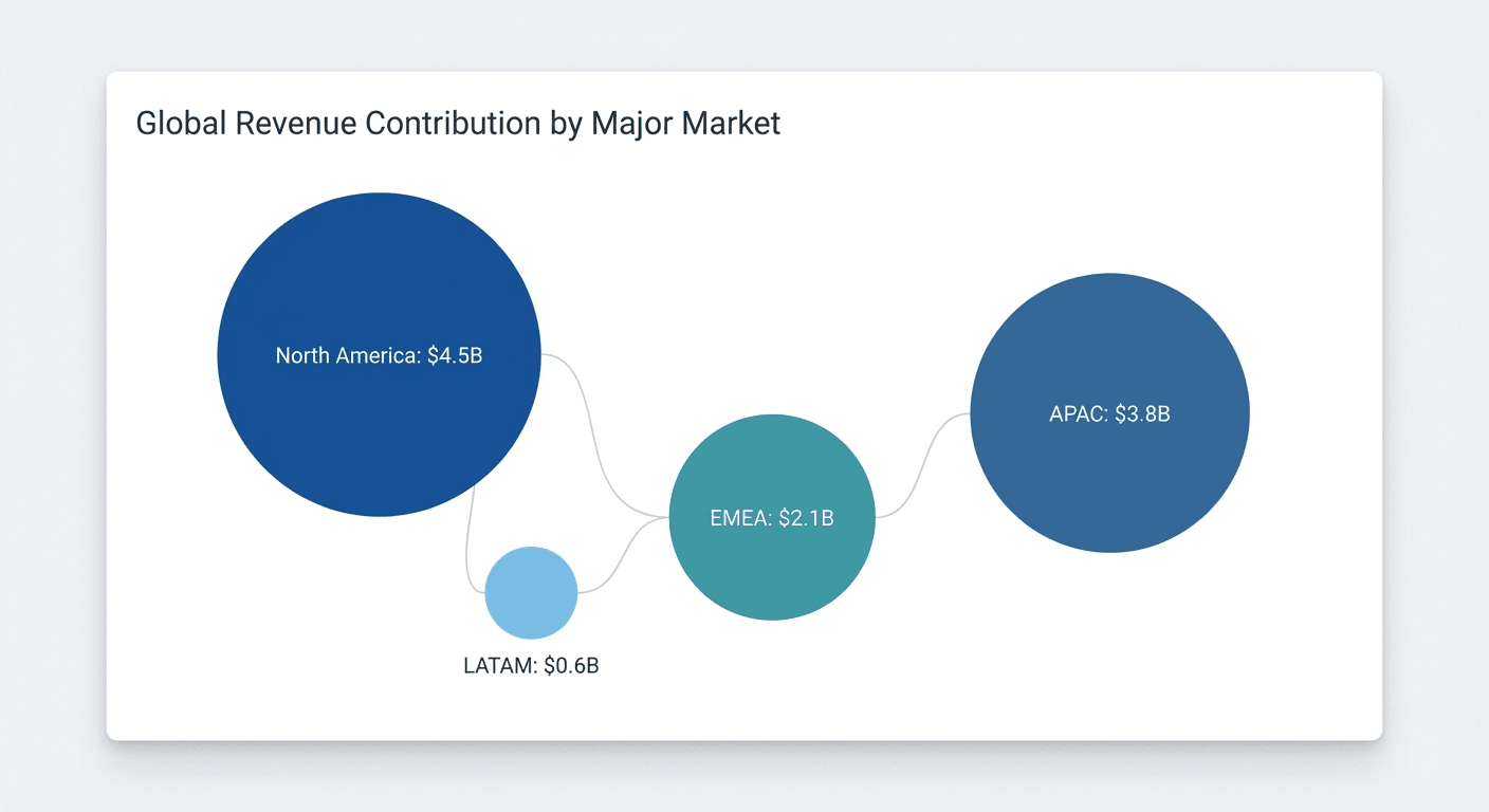
Dorling cartograms
Circles replace regions. That’s the point.
Regions are replaced by circles sized by the data variable. Geography is abstracted entirely. Viewers must rely on labels or color to identify regions. Use these when the data message matters more than geographic context, or when presenting to audiences unfamiliar with the base geography.
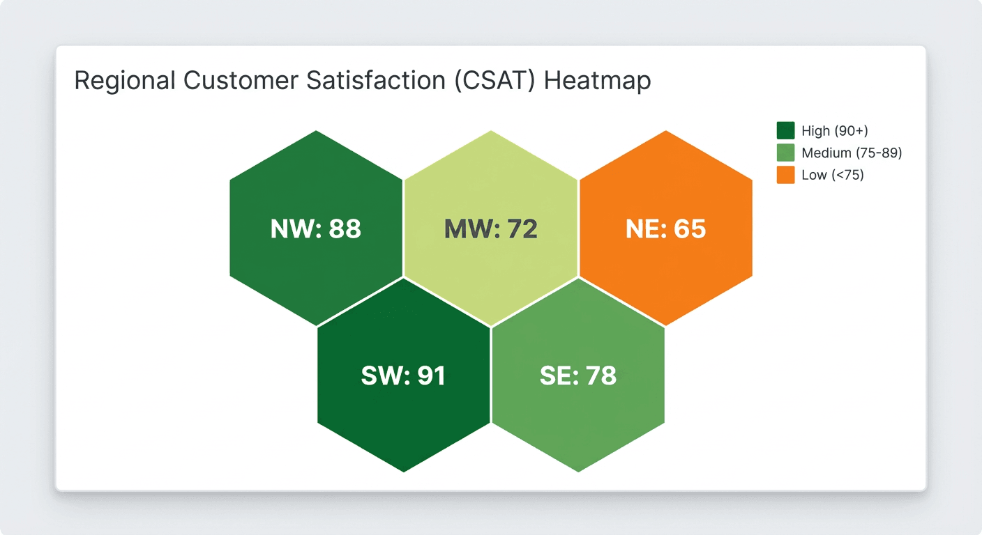
Tile grid cartograms
These look neat and orderly because they are.
Regions are replaced by equal-sized squares or hexagons arranged in a grid approximating the original geography. Each unit represents one region regardless of actual land area. Tile grids are easy to scan and label, but they don’t encode magnitude through area, so you typically rely on color (or a label) to carry the value.
Best practices for cartogram charts
If you’ve ever watched someone misread a cartogram in a meeting, these will feel familiar.
Reference map or legend
Always include a reference map or legend. Without a standard map for comparison, viewers unfamiliar with the geography can’t identify which region is which. The “aha” moment depends on recognizing the distortion.
Direct labels
Label key regions directly on the chart. Relying on color legends forces viewers to look away from the visual. Direct labels on the largest and most distorted regions reduce cognitive load.
Use totals, not rates
Use cartograms for totals, not rates. Encoding a rate (per capita income, infection rate per 100,000) as area creates mathematical incoherence. A region with high per capita income but small population will appear large, implying it contributes more to the total than it actually does.
Validate adjacency
If using contiguous cartograms, validate that the algorithm preserved adjacency. Some algorithms introduce topological errors where regions that should be neighbors become separated. Spot-check a few known adjacencies before publishing.
Avoid dominant regions
Avoid cartograms when one region dominates. If one region contains more than half the total value, most other regions will shrink to near-invisibility. Your “map” becomes a single shape with crumbs around it.
Connect to live data
If your team builds cartogram charts in disconnected tools, governance can get messy fast. One team exports data on Monday, another team refreshes on Thursday, and suddenly you have multiple versions of the same “regional revenue” story floating around. Keeping cartograms connected to live, governed data sets is the only real fix.
Cartogram chart examples
Population cartogram of US states
A policy team needs to communicate that California, Texas, Florida, and New York together account for a large share of the US population. On the cartogram, these four states balloon to dominate the map while geographically large but sparsely populated states, like Montana, Wyoming, or Alaska, shrink to near-invisibility.
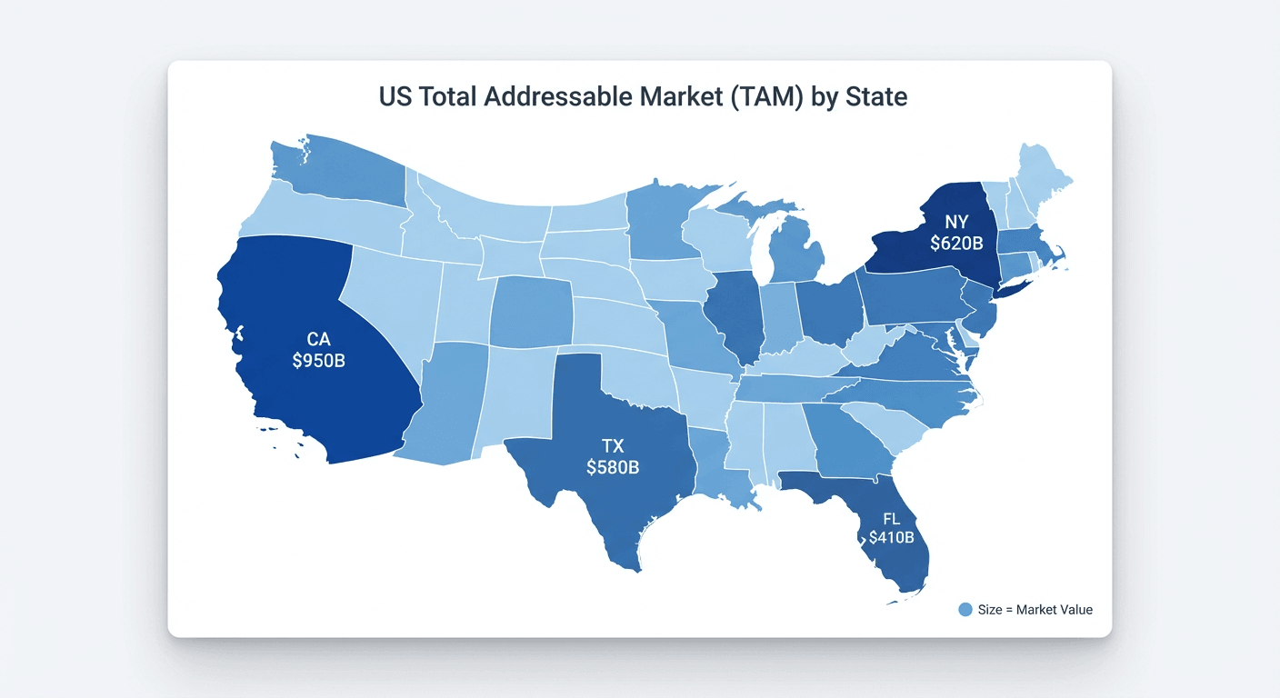
On a standard map, Alaska appears massive and California appears moderate. The geography fights the story. That’s exactly the problem cartograms were built to solve.
Revenue by sales territory
This is the moment cartograms start to feel practical.
A sales operations team needs to justify reallocating headcount from large geographic territories to small but high-revenue urban territories. Urban territories (Northeast corridor, Bay Area, Chicago metro) expand dramatically while rural territories (Mountain West, Great Plains) shrink despite covering more land. A standard territory map would show rural territories as dominant, reinforcing the status quo.
In practice, this is also where interactive dashboards help. A regional marketing manager might filter the same cartogram by product line or campaign, while an executive toggles between revenue, customer count, and headcount to sanity-check the story in real time.
How to create a cartogram chart
Spreadsheets aren’t built for this. Really.
Cartograms require specialized algorithms that most spreadsheet tools don’t support natively. You can’t build a true contiguous cartogram (the “rubber-sheet” style distortion) in Excel without external add-ins or pre-processed data. You can still create a tile grid cartogram using Excel’s cell formatting.
For a tile grid approach in Excel:
- Create a table with columns for State, Column coordinate, Row coordinate, and Value.
- Assign row/column numbers that approximate the map layout (templates exist online for US state grids).
- Resize worksheet cells to be perfect squares.
- Type state abbreviations in cells corresponding to the map layout.
- Apply conditional formatting color scales to the values.
For true contiguous or Dorling cartograms, BI platforms that support cartogram charts can save you a lot of prep work. Domo includes cartogram chart visualization options inside its BI platform, so analysts can build a cartogram chart tied directly to governed data sets without exporting data into separate mapping or geographic information system (GIS) applications. The usual failure mode here is simple: you build a beautiful cartogram once, then keep screenshotting it for slides, and the numbers quietly drift.
If you’re preparing geographic data sets for a cartogram chart, keeping transformation and validation close to the visualization helps. In Domo, data engineers often use Magic Transform (Structured Query Language (SQL) or no-code) to normalize region identifiers, enforce consistent metrics, and shape the data set so the cartogram chart renders cleanly.
After generating any cartogram, verify that the area of each region correlates with your input data. Spot-check the largest and smallest regions to confirm they match expectations.
Limitations and alternatives
Cartograms trade precise location for magnitude. Human perception of area is also imprecise, so cartograms support ranking more than precise measurement.
When cartograms don’t fit, consider these alternatives:
- Choropleth map: Better for rate-based data where geographic accuracy matters
- Bubble map overlay: Better when you want to show totals without distorting boundaries
- Bar chart: Better when geographic context is irrelevant and you only need to rank regions
Choropleths preserve geography and encode rates. Cartograms distort geography and encode totals. Bubble maps preserve boundaries while still encoding magnitude, making them less visually dramatic but more geographically accurate. Which one you reach for first says something about what question you’re actually trying to answer.
If you’re working in an environment where executives expect real-time answers, stale exports become a quiet problem. A cartogram chart connected to live operational data can stay current, and AI-driven insights (like anomaly detection) can flag when a region suddenly deviates from the pattern you expect, right where you’re already looking.