Guide to AWS Redshift Architecture

Amazon Redshift has become one of the most widely adopted cloud data warehouses, particularly for organizations already operating inside the AWS ecosystem. It sits at the where traditional data warehousing concepts meet modern cloud-native architecture, offering scalable analytics without the operational overhead of managing physical infrastructure. 

For data teams, analytics engineers, and business leaders alike, understanding how Redshift works under the hood is key to using it effectively, controlling costs, and designing well-performing analytics pipelines.

This guide provides a comprehensive, high-level overview of AWS Redshift architecture. It focuses on how Redshift is structured, how its components interact, and why those architectural decisions matter. By the end, you should have a clear mental model of how data flows through Redshift, how compute and storage are handled, and how Redshift fits into a broader analytics stack.

What Amazon Redshift is and where it fits

Amazon Redshift is a fully managed, columnar data warehouse designed for large-scale analytical workloads. Unlike transactional databases that are optimized for frequent inserts, updates, and deletes, Redshift is built for reading and aggregating large volumes of data across many rows and columns. Typical use cases include business intelligence reporting, historical trend analysis, and powering dashboards for operational and executive decision-making.

From an architectural standpoint, Redshift borrows heavily from traditional massively parallel processing (MPP) data warehouse designs. At the same time, it incorporates cloud-native concepts such as elastic scaling, managed storage, and tight integration with object storage in Amazon S3. This hybrid approach allows Redshift to feel familiar to data warehouse practitioners while still benefiting from the flexibility of the cloud.

Redshift is often positioned as the analytical core of an AWS-based data stack. Data commonly lands first in S3 from operational systems, SaaS tools, or streaming platforms, then gets transformed and loaded into Redshift for querying. BI tools, data science notebooks, and downstream applications connect to Redshift to consume curated, analytics-ready data.

High-level overview of Redshift architecture

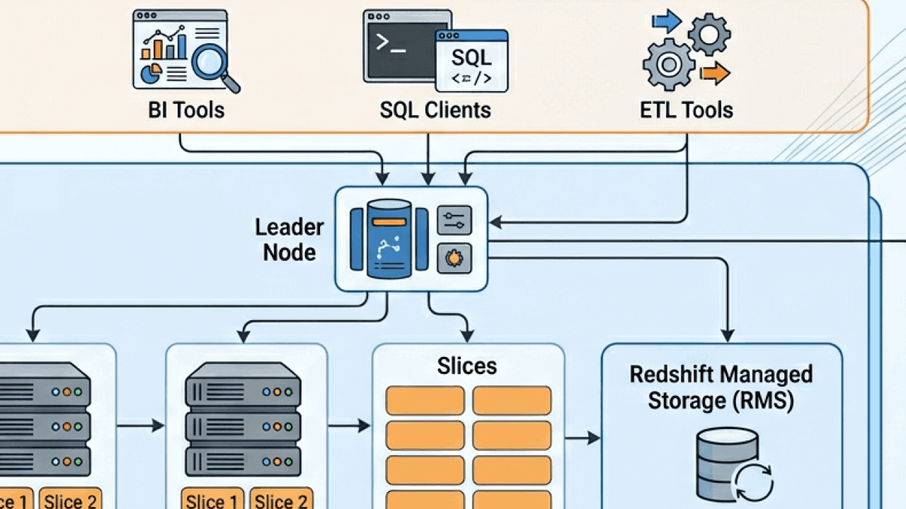
At a high level, Amazon Redshift consists of a cluster made up of a leader node and one or more compute nodes. These nodes work together to store data, execute queries, and return results to people and applications. Around this core cluster are supporting services for storage, networking, security, and management that are largely abstracted away from people.

The key idea behind Redshift’s architecture is the separation of concerns. Query planning and coordination are handled by the leader node, while data storage and query execution are distributed across compute nodes. This allows Redshift to process large analytical queries in parallel, significantly improving performance compared to single-node systems.

In more recent iterations, Redshift has evolved beyond the original cluster-centric model by introducing features like managed storage, concurrency scaling, and serverless options. These additions further decouple compute from storage and make the platform more elastic, while preserving the same underlying architectural principles.

The role of the leader node

The leader node acts as the brain of a Redshift cluster. It doesn’t store people’s data or perform heavy query processing. Instead, it’s responsible for parsing SQL queries, generating optimized query execution plans, and coordinating work across the compute nodes.

When someone submits a query to Redshift, it first arrives at the leader node. The leader node parses the SQL, validates it against the system catalog, and determines how to best execute it in parallel. This includes deciding which compute nodes should process which portions of the data and how intermediate results should be combined.

The leader node also aggregates results returned from compute nodes before sending the final output back to the client. Because of this coordinating role, the performance and stability of the leader node are critical, especially in environments with many concurrent users or complex queries.

Although people rarely interact with the leader node directly, understanding its function helps explain certain behaviors, such as query queuing or the impact of concurrency on overall system performance.

Compute nodes and massively parallel processing

Compute nodes are where the actual data lives and where much of the query execution happens. Each compute node stores a subset of the total data and processes queries on that subset independently and in parallel with other nodes.

This massively parallel processing model is what allows Redshift to handle very large data sets efficiently. Instead of scanning billions of rows on a single machine, Redshift divides the work across many nodes, each scanning a fraction of the data at the same time.

Within each compute node, data is further divided into slices. A slice represents a portion of a node’s CPU, memory, and disk resources. Queries are executed at the slice level, which enables even finer-grained parallelism. The number of slices per node depends on the node type and size.

As data volumes grow, additional compute nodes can be added to a cluster, allowing Redshift to scale horizontally. While scaling isn’t instantaneous and does require some planning, the architectural model makes it relatively straightforward to increase capacity as analytics demands evolve.

Node types and deployment models

Redshift offers different node types designed for different workload profiles. Historically, these included dense compute nodes and dense storage nodes, allowing customers to choose between higher CPU-to-storage ratios or more cost-effective storage-heavy configurations.

More recently, Amazon introduced RA3 nodes, which fundamentally changed how Redshift handles storage. With RA3, compute nodes use fast local storage for frequently accessed data while easily offloading less frequently used data to managed storage in S3. This allows compute and storage to scale more independently than before.

From an architectural perspective, RA3 nodes reduce the tight coupling between data volume and cluster size. Instead of adding compute nodes solely to gain more disk space, organizations can scale compute for performance and rely on managed storage for capacity.

This evolution reflects a broader trend in cloud data platforms toward separating compute and storage, improving both flexibility and cost efficiency.

Data storage and columnar design

One of the defining characteristics of Redshift is its columnar storage format. Unlike row-based databases that store all columns of a row together, columnar databases store each column separately.

This design is particularly well-suited for analytical queries, which often scan only a subset of columns across many rows. By reading only the columns required for a query, Redshift can dramatically reduce disk I/O and improve query performance.

Columnar storage also enables high levels of compression. Because values within a column are often similar, Redshift can apply compression encodings that reduce storage footprint and further speed up data scans. Compression is handled automatically in most cases, simplifying management for users.

Data is stored on disk in immutable blocks. When data is updated or deleted, Redshift doesn’t modify existing blocks but instead marks rows as deleted and writes new blocks as needed. This approach aligns with analytical workloads but also introduces periodic maintenance operations, such as vacuuming, to reclaim space and optimize performance.

Data distribution and its impact

Data distribution is a core concept in Redshift architecture and has a significant impact on query performance. Because data is spread across compute nodes, how that data is distributed determines how much data needs to be moved during query execution.

Redshift uses distribution styles to control how rows of a table are assigned to nodes. The goal is to minimize data shuffling during joins and aggregations. When related data is co-located on the same nodes, queries can be executed locally without expensive network transfers.

Although modern Redshift has become more forgiving with features like automatic table optimization, understanding distribution remains important for designing scalable schemas. Poor distribution choices can lead to data skew, where some nodes do much more work than others, slowing down queries and wasting resources.

From an architectural perspective, distribution is one of the key ways Redshift translates logical table design into physical execution efficiency.

Query execution lifecycle

When a query runs in Redshift, it follows a multistage lifecycle that reflects the platform’s distributed architecture. After the leader node generates a query plan, it breaks that plan into steps that can be executed in parallel across compute nodes.

Each compute node processes its assigned portion of the data, performing operations such as scans, filters, joins, and aggregations. Intermediate results may be exchanged between nodes if required by the query plan, for example, when joining tables that are distributed differently.

Once the compute nodes finish their work, partial results are sent back to the leader node. The leader node then performs any final aggregation or sorting before returning the complete result set to the client.

This pipeline-oriented execution model allows Redshift to handle complex analytical queries efficiently, even at a very large scale. At the same time, it makes query performance sensitive to factors like data distribution, node balance, and concurrency.

Workload management and concurrency

In real-world environments, Redshift rarely runs a single query at a time. Instead, multiple people and applications submit queries concurrently, each with different priorities and resource requirements.

Redshift addresses this through workload management. Queries are assigned to queues, each with configurable limits on concurrency and memory usage. This helps prevent resource contention and ensures that critical workloads receive sufficient resources.

From an architectural standpoint, workload management sits between the query interface and the execution engine. It acts as a traffic controller, deciding when queries are allowed to run and how resources are allocated.

Newer Redshift features, such as automatic workload management and concurrency scaling, further abstract these concerns by dynamically adding transient compute capacity when demand spikes. This allows organizations to support many concurrent users without permanently overprovisioning their clusters.

Networking and security architecture

Redshift clusters are deployed within Amazon Virtual Private Cloud environments, allowing fine-grained control over network access. Clusters can be isolated in private subnets and accessed only through approved endpoints.

Communication between clients and Redshift is encrypted using standard protocols, and data at rest is encrypted by default using AWS-managed or customer-managed keys. These security features are deeply integrated into the architecture, rather than layered on as optional add-ons.

Redshift also integrates with AWS Identity and Access Management for authentication and authorization. This enables centralized control over who can access the cluster and what actions they can perform, aligning data warehouse security with broader cloud governance practices.

Integration with the AWS data ecosystem

One of Redshift’s architectural strengths is its tight integration with other AWS services. Amazon S3 plays a particularly important role, acting as both a staging area for data ingestion and, in modern configurations, a managed storage layer.

Data can be loaded into Redshift efficiently using bulk operations from S3, taking advantage of parallelism and high-throughput networking. Conversely, query results can be unloaded back to S3 for downstream processing or sharing.

Redshift also integrates with AWS services for streaming data, orchestration, and monitoring. These integrations allow Redshift to function as part of a larger, modular data architecture rather than a standalone system.

Redshift Spectrum and external data

Redshift Spectrum extends the platform’s architecture beyond the boundaries of the cluster by allowing queries to run directly against data stored in S3. Instead of loading all data into Redshift tables, individuals can define external schemas that reference files in object storage.

When a query accesses external data, Redshift delegates the scan to Spectrum’s distributed processing layer, then combines the results with data stored in the cluster. This approach allows organizations to query massive data sets without incurring the cost of loading and storing them in the warehouse.

Architecturally, Spectrum blurs the line between data lake and data warehouse. It enables a hybrid model where frequently accessed, curated data lives in Redshift, while large volumes of raw or historical data remain in S3.

Operational considerations and maintenance

Although Redshift is fully managed, its architecture still imposes certain operational considerations. Tasks such as monitoring disk usage, managing table bloat, and tuning workloads remain important for maintaining performance over time.

Maintenance operations like vacuuming and analyzing tables help ensure that the physical storage layout remains efficient and that the query planner has accurate statistics. While many of these tasks can be automated, understanding why they’re necessary requires an appreciation of Redshift’s underlying storage model.

From an architectural standpoint, these maintenance pressures are a natural consequence of Redshift’s append-oriented, columnar design and its focus on analytical performance.

How Redshift architecture supports analytics at scale

Taken as a whole, AWS Redshift architecture is designed to balance performance, scalability, and manageability. Its MPP foundation enables fast query execution on large data sets, while its cloud-native enhancements reduce operational complexity.

By separating query coordination, execution, and storage concerns, Redshift can evolve incrementally without forcing anyone to redesign their data models. Features like managed storage, concurrency scaling, and external querying build on the same core principles rather than replacing them.

For organizations building modern analytics platforms, Redshift’s architecture provides a flexible foundation that can support everything from traditional BI reporting to more advanced, data-driven applications.

Final thoughts

Understanding AWS Redshift architecture is less about memorizing components and more about developing an intuition for how data and queries move through the system. When you grasp how leader nodes, compute nodes, storage, and parallel execution fit together, it becomes much easier to design efficient schemas, diagnose performance issues, and plan for growth.

As analytics needs continue to evolve, Redshift’s architecture has shown a clear trajectory toward greater flexibility and deeper integration with the broader data ecosystem. For teams already invested in AWS, it remains a powerful and relevant option for large-scale analytics, provided its architectural strengths and trade-offs are well understood.